where [Ca]o = 1.2 mM and [Ca,1]in refers to intracellular calcium in pool number 1 (see the description for the calcium dynamics). Initial [Ca]in was set to 50 nM.
Here we provide a detailed description of the model used for the simulation of Local Field Potentials (LFPs) in the rat hippocampal Dentate Gyrus (DG).
The model is built in three levels of complexity:
Compartmental transmembrane currents and potentials were calculated using the GENESIS simulator (Bower and Beeman, 1998), with a time step of 10 μs. Calculation of LFPs was done using a customary software written in MATLAB.
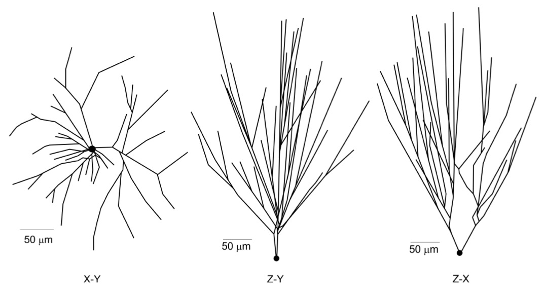
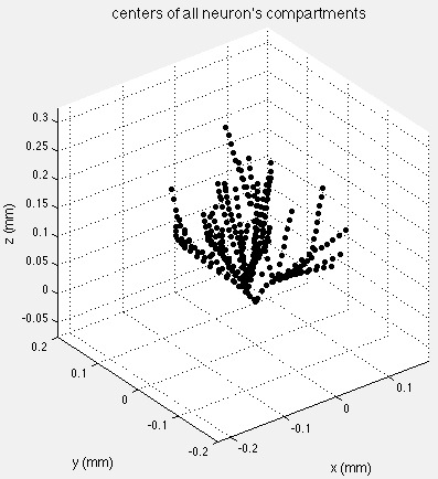
The prototype model neuron was built with an average dendritic branching pattern, and total dendritic length obtained from detailed morphometric studies (Bannister and Larkman, 1995 a,b; Trommald et al., 1995). The 3D morphology of the neuron was simulated using 335 compartments distributed among soma and dendritic trees. 2D projections of the model neuron are shown in the figure below. Total effective area of the neuron was 11679 μm2 including spine area. The soma compartment is spherical, all the others are cylindrical.
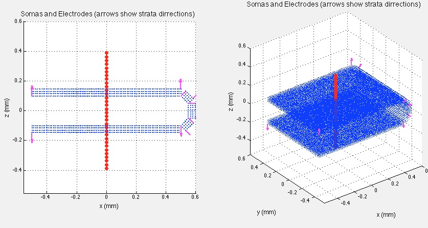
The Dentate Gyrus region was modeled as an aggregate preserving experimentally observed cell density of 100 neurons in a 50x50 μm lattice. The antero-posterior, latero-medial, and ventro-dorsal dimensions of the aggregate were 1x0.8x0.3 mm, respectively, corresponding to 50384 morphologically identical model neurons. The dimensions and cell number of the aggregate estimate the actual values for the Dentate Gyrus region. The spatial distribution of neurons was made with their somata arranged in a realistic manner of 4 equal layers. We simulated Dentate Gyrus - like configuration with 5 differently orientated neuronal sections (horseshoe-like, see figure below): 2 opposite parallel sections and 3 others with different angles (45°, 90°, and 135°) to form gyrus. The neurons' main axis always was orthogonal to the corresponding section. Neurons in the layers have some random deviation of 2 μm from the grid.
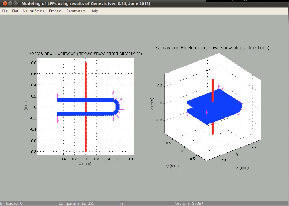
A set of 64 recording points 25 μm apart in a vertical track (red dots mark positions of the recording points) spanning from 800 μm above to 800 μm below the Granular cells stratum was placed at the center of the population in parallel to the somatodendritic axis. The value of the field potential measured at each point was calculated as follows:
The activity of a multi-compartmental neuron (see below) produces membrane currents, which in turn generate LFP. Simulation of the dynamics of a neuron in Genesis provides membrane currents for all compartments: Ij(t), (j = 1, 2,..., M) [measured in Amperes], where M = 335 for our Dentate Gyrus neuron. Thus we can consider that the total membrane current source density, J(t,x), is given by point current sources corresponding to M compartments:
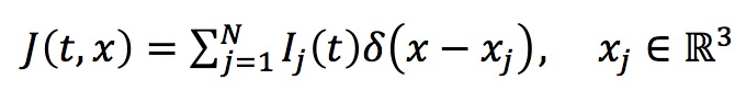
where xj are the spatial positions [measured in meters] of the compartments related to the soma's compartment placed in the origin.
We assume a homogenous conductive medium with constant conductivity σ = 0.3 S/m. Then the electric potential created by a single neuron can be modeled by the Poisson's equation:
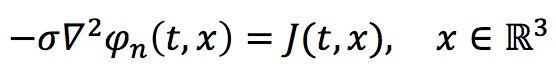
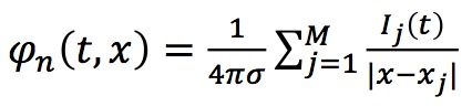
Solution of this equation (in the sense of distributions) is given by
Let us now assume that we have N identical neurons distributed in several layers (four by default) within a neuronal section.
Then the potential produced by this neuronal section is
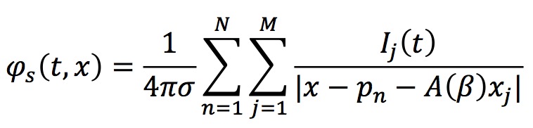
where pn is the absolute position of the soma of the n-th neuron within the section and
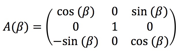
is the rotating matrix (beta is the angle of rotation).
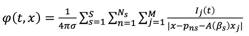
For a multi-section configuration (as in the figure above) the potential is given by
We assume that the electric potential is recorded by K electrodes placed in positions xk. Then twe obtain
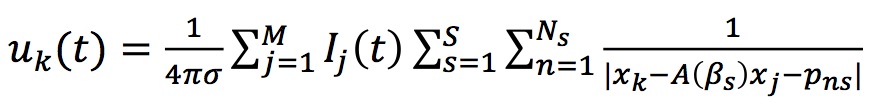
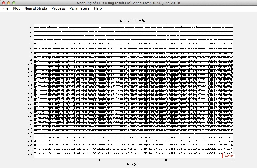
Using Ij(t) provided by Genesis (see below) we can obtain simulated LFPs in the Dentate Gyrus. The following figure shows typical LFP-traces.
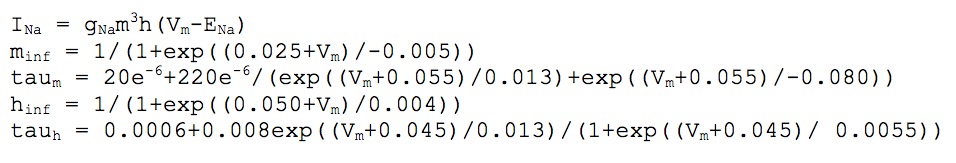
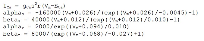
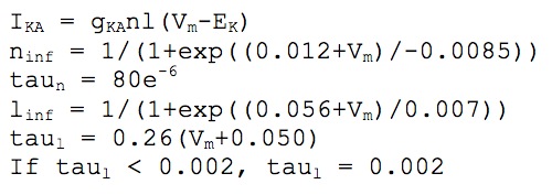
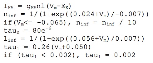
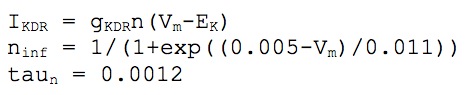
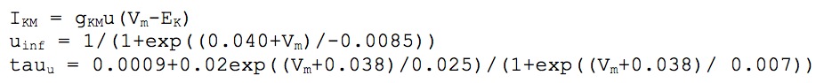
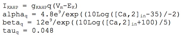
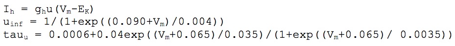
We used twelve types of ionic channels to simulate the active properties of the cellular membrane: two kinds of fast transient sodium (Na+) for the axon and soma-dendrites, two of calcium (Ca++) high and low thereshold, and seven potassium (K+) currents: two delayed rectifier (DR), (somatodendritic and axonic), small persistent muscarinic (M), two A-type transient, (proximal and distal), short duration [Ca] and voltage dependent (C) and long duration [Ca] dependent (AHP). We also modeled a hyperpolarization activated current (h). Kinetics was derived from Warman et al. (1994), Hoffman et al. (1997), Migliore et al. (1999), Colbert and Pan (2002), and Traub et al. (2003).
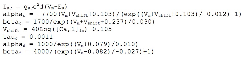
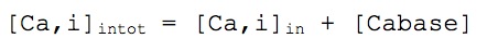
As described by Warman et al. (1994) and Borg-Graham (1998), the [Ca]i was simulated as two different Ca pools with different time constants, tau1 = 0.9 ms for the calculation of ECa and modulating the C-type K+ current, and tau2 = 1 s for the AHP-type K+ current, as follows:

where taui is the removal time constant in the i-th calcium pool, fi the fraction of Ca influx affecting the i-th pool (f1=0.7, f2=0.024), w is the thickness of the diffusion shell (1 μm in compartments with diameter > 2 μm, or its diameter on thinner dendrites), A is the compartment area, z is the valence of the calcium ion and F is the Faraday's constant.
The extracellular concentration ([Ca]o) is considered constant and equal to 1.2 mM. The initial (rest) intracellular concentration [Cabase] is 50 nM.
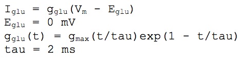
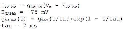
The synaptic stimulation was simulated by activation of excitatory synaptic channels of AMPA type and inhibitory GABAA type conductances. The conductance of all synaptic channels was modeled as alpha functions, described below.