Description

This script reproduces some results of the study of simulated LFPs.

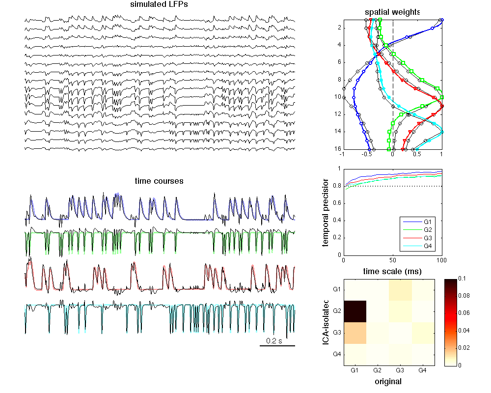
It corrsponds to Fig. 2 for Makarova et al. (2011). Parallel Readout of Pathway-Specific Inputs to Laminated Brain Structures.

Frontiers in Systems Neuroscience.

After reviewer's revision. July 21, 2011.

Contents

Load simulated data

close all
clear all
cd('/Users/valeri/Dropbox/Julia/Frontiers Neuroscience 2011/Revision');
path(path,'./MatFunc');
path(path,'/Users/valeri/Dropbox/work/LFPanalysis/MatFunc/');

% Original separate generators
load('./DATA/G1_ICA.mat'); os = G.s(1,:); oM = G.V(:,1);
load('./DATA/G2_ICA.mat'); os = [os; G.s(1,:)]; oM = [oM G.V(:,1)];
load('./DATA/G3_ICA.mat'); os = [os; G.s(1,:)]; oM = [oM G.V(:,1)];
load('./DATA/G4.mat');     os = [os; G.s(1,:)]; oM = [oM G.V(:,1)];

% ICA-isolated LFP-generators
load('./DATA/G1+G2+G3+G4.mat'); s = G.s;

Fs = Args.Fs;
N = size(s,1);
t = ((1:size(s,2))-1)/Fs;

Evaluate the Cross-Contamination Index

xShift = 2000; % remove transient part
os = CenterZeroValue(os, xShift);
s  = CenterZeroValue(s, xShift);
s  = AdjustLoadings(s, os, xShift);
s  = CenterZeroValue(s, xShift);

CCind = GeneratorCrossContamination(s(:,xShift:end),  os(:,xShift:end));
CCind = CCind - eye(size(CCind));

Evaluate temporal precision

maxScale = 100;
wname  = 'haar';
ntw = 3;
Ratio = 1;
scales = 2:2:(maxScale/Ratio);
for k = 1:N,
    WC{k} = wcoher(os(k,xShift:end),s(1,xShift:end),scales,wname,'ntw',ntw);
end

Plot Figure 2

XLm = [1 2.55];

h = figure('color','w','position',[100 100 1000 800]);

subplot('position',[0.05 0.6 0.55 0.37])
PlotEEG(LFP, Fs, 'e')
xlim(XLm)
axis off
title('simulated LFPs','FontSize',14)

subplot('position',[0.05 0.12 0.55 0.4])
Dy = 500;
YY = [0 -0.4 -2.2 -2.7];
clr = [0.6 0.6 1; 0.6 1 0.6; 1 0.6 0.6; 0.6 1 1];
hold on
for k = 1:N,
    plot(t, os(k,:) + Dy*YY(k), 'color', clr(k,:), 'LineWidth', 2);
    plot(t,  s(k,:) + Dy*YY(k), 'k')
end

Dx = 0.1*round(diff(XLm));
ylm = get(gca, 'Ylim');
plot([XLm(2),XLm(2)-Dx],ylm(1)*[1 1],'k','LineWidth',2)
text(XLm(2)-Dx*0.8, ylm(1) + 0.03*diff(ylm),[num2str(Dx) ' s'],'FontSize',12)
xlim(XLm)
title('time courses','FontSize',14)
axis off

subplot('position',[0.7 0.62 0.2 0.33])
plot(G.V, 1:16,'ko-')
hold on
PlotLoadingsYX(oM)
xlim([-1 1])
title('spatial weights','FontSize',14)

subplot('position',[0.7 0.35 0.2 0.22])
clr = 'bgrcmyk';
for k = 1:N
    plot(Ratio*scales,mean(abs(WC{k}),2),[clr(k) '-'], 'LineWidth',1);
    hold on
end
plot(Ratio*[scales(1), scales(end)],0.8*[1 1],'k:','LineWidth',2);
legend({'G1','G2','G3','G4'},'location','best')
axis([0 scales(end)*Ratio 0 1])
xlabel('time scale (ms)','FontSize',14)
ylabel('temporal precision','FontSize',14)

subplot('position',[0.7 0.07 0.25 0.22])
imagesc(CCind, [0 0.1])
colorbar
m = zeros(64,3);
m(:,1) =  1.1 - ((1:64) - 35)/30;
m(:,2) =  1 - ((1:64) - 5)/30;
m(:,3) =  1 - (1:64)/25;
m(m > 1) = 1; m(m < 0) = 0;
colormap(m)
ylabel('ICA-isolated','FontSize',14)
xlabel('original','FontSize',14)
set(gca,'YTick',1:N); set(gca,'YTickLabel',{'G1','G2','G3','G4'})
set(gca,'XTick',1:N); set(gca,'XTickLabel',{'G1','G2','G3','G4'})

Published with MATLAB® 7.11