An example showing the basic usage of the wICA algorithm

This code is for illustration of the method described in: N.P. Castellanos and V.A. Makarov (2006). "Recovering EEG brain signals: Artifact suppression with wavelet enhanced independent component analysis" J. Neurosci. Methods 158, 300-312.

Requirements: runica from EEGLAB toolbox, and rwt - Rice Wavelet Toolbox (both freely available in internet).

This code is copyright © by the authors, and we hope you acknowledge our work. We distribute it in the hope that it will be useful, but without any warranty.

Author: Valeri A. Makarov e-mail: vmakarov@mat.ucm.es

http://www.mat.ucm.es/~vmakarov

2006

Contents

Reset environment

close all
clear all

Read test data

Fs = 256;  % Sampling frequency in Hz
[Data, ChanTitels, FileName] = ReadTruScan_ascii('./Data/test1.tdt');

Conventional notch filter (you may add more)

This is an optional step (suppress 50Hz noise)

Fnyq  = Fs/2;
F_notch = 50; % Notch at 50 Hz
[b,a] = iirnotch(F_notch/Fnyq, F_notch/Fnyq/20);
Data  = filtfilt(b,a, Data);

Conventional High Pass Filter

This is an optional step (suppress low <4Hz frequency noise)

F_cut = 4;
[b,a] = ellip(1, 0.5, 20, F_cut/Fnyq, 'high');
Data  = filtfilt(b,a, Data);

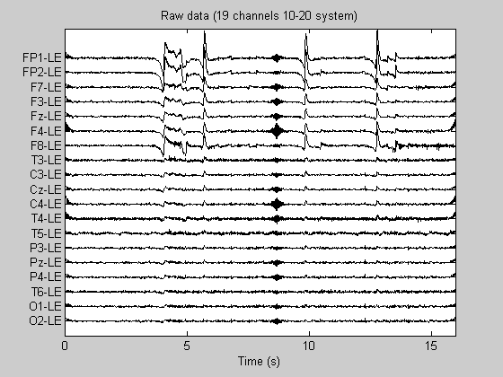
Remove mean values from the channels and plot raw data

Data  = detrend(Data,'constant');
% Transpose the data matrix to get (channel x time) orientation
Data = Data';
figure;
PlotEEG(Data, Fs, ChanTitels, 200, 'Raw data (19 channels 10-20 system)');

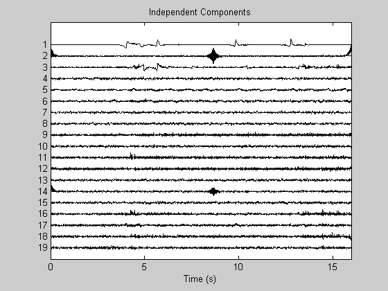
Find independent components

EEGLAB is required!!! You can also use other algorithms, e.g. fastICA. Note: the use of long (in time) data sets reduces the algorithm performance see for details the abovementioned paper.

[weight, sphere] = runica(Data, 'verbose', 'off');
W = weight*sphere;    % EEGLAB --> W unmixing matrix
icaEEG = W*Data;      % EEGLAB --> U = W.X activations
figure;
PlotEEG(icaEEG, Fs, [], [], 'Independent Components');
xlabel('Time (s)')

Inverting negative activations: 1 2 -3 4 5 6 -7 8 9 -10 11 12 -13 -14 15 -16 17 18 -19 

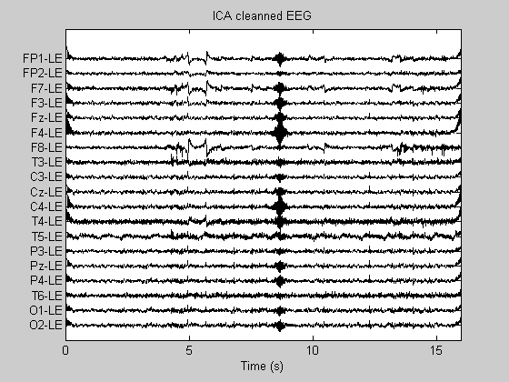
Common ICA artifact suppression method

Remove artifact components and rebuild signals

An input dialog will be open, where you should enter the ICs to be removed (those with artifacts)

answer  = inputdlg({'Artifact ICs'},'Components to remove',1);
ArtICs = str2num(answer{1});
disp(['Suppressed components: ' answer{1}]);
icaEEG1 = icaEEG;
icaEEG1(ArtICs, :) = 0;          % suppress artifacts
Data_ICA = inv(W)*icaEEG1;       % rebuild data
figure;
PlotEEG(Data_ICA, Fs, ChanTitels, 100, 'ICA cleanned EEG');

Suppressed components: 1

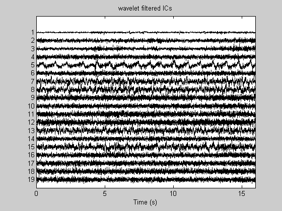
wICA artifact rejection

Rice Wavelet Toolbox (rwt) is required!!!

You can also tune the third argument, or/and provide (in the second argument) the numbers of the components to be processed e.g. [1:4,7] (in the example we process all 19 components).

[icaEEG2, opt]= RemoveStrongArtifacts(icaEEG, (1:19), 1.25, Fs);
Data_wICA = inv(W)*icaEEG2;
figure;
PlotEEG(icaEEG2, Fs, [], [], 'wavelet filtered ICs');
figure;
PlotEEG(Data_wICA, Fs, ChanTitels, 100, 'wICA cleanned EEG');

The component #1 has been filtered
The component #2 has been filtered
The component #3 has been filtered
The component #4 has been filtered
The component #5 has passed unchaneged
The component #6 has been filtered
The component #7 has passed unchaneged
The component #8 has passed unchaneged
The component #9 has been filtered
The component #10 has been filtered
The component #11 has been filtered
The component #12 has been filtered
The component #13 has passed unchaneged
The component #14 has been filtered
The component #15 has passed unchaneged
The component #16 has been filtered
The component #17 has been filtered
The component #18 has been filtered
The component #19 has been filtered

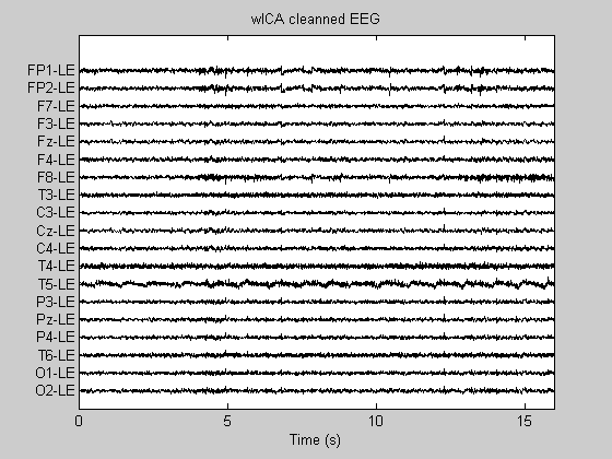
Make a comparative plot

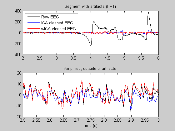
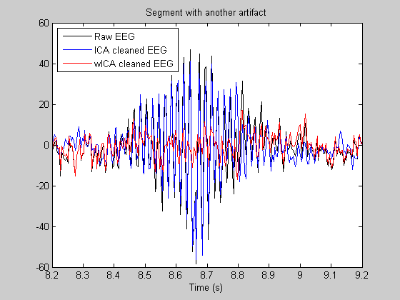
We plot a segment with (ocular) artifacts and an artifact-free segment. Note: in the artifact-free segment a good artifact suppression method should conserve (not perturb) the original EEG signal. Third graph shows one more example.

figure
subplot(2,1,1);
T1 = 2; T2 = 6;
nT1 = T1*Fs; nT2 = T2*Fs;
plot((nT1:nT2)/Fs, Data(1,nT1:nT2),'k',(nT1:nT2)/Fs, Data_ICA(1,nT1:nT2),'b',...
    (nT1:nT2)/Fs, Data_wICA(1,nT1:nT2),'r');
legend({'Raw EEG','ICA cleaned EEG','wICA cleaned EEG'},'Location','NorthWest');
title('Segment with artifacts (FP1)')
subplot(2,1,2);
T1 = 2.5; T2 = 3;
nT1 = T1*Fs; nT2 = T2*Fs;
plot((nT1:nT2)/Fs, Data(1,nT1:nT2),'k',(nT1:nT2)/Fs, Data_ICA(1,nT1:nT2),'b',...
    (nT1:nT2)/Fs, Data_wICA(1,nT1:nT2),'r');
title('Amplified, outside of artifacts')
xlabel('Time (s)')
figure
T1 = 8.2; T2 = 9.2;
nT1 = T1*Fs; nT2 = T2*Fs;
plot((nT1:nT2)/Fs, Data(1,nT1:nT2),'k',(nT1:nT2)/Fs, Data_ICA(1,nT1:nT2),'b',...
    (nT1:nT2)/Fs, Data_wICA(1,nT1:nT2),'r');
legend({'Raw EEG','ICA cleaned EEG','wICA cleaned EEG'},'Location','NorthWest');
title('Segment with another artifact')
xlabel('Time (s)')

Warning: Integer operands are required for colon operator when used as index
Warning: Integer operands are required for colon operator when used as index
Warning: Integer operands are required for colon operator when used as index

Published with MATLAB® 7.2